Recap

統整一下前面的幾個章節: 對於 batch & supervised binary classification 的問題而言， $g \approx f \iff E_{\text{out}} \approx 0$ 而後者可以經由兩個階段來取得

training: $E_{\text{in}} \approx 0$
testing: $E_{\text{out}} \approx E_{\text{in}}$

Trade-off on M

現在我們可以歸納出兩個問題:

如果確保 $E_{\text{in}}$ 和 $E_{\text{out}}$ 足夠接近？
如何讓 $E_{\text{in}}$ 足夠小？

而這兩個問題都和 $M$ (size of $\mathcal{H}$ ) 有關:

small $M$ $M$ :
1. Yes: 誤差 $\le 2M\exp(\cdots)$
2. No: 選擇太少
large $M$ $M$ :
- No
- Yes: 選擇很多

我們要如何選擇剛好的 $M$ 呢？

Effective Number of Lines

Union Bound is Over-estimated

在 Lecture 4，我們用了 union bound 的方法來計算誤差的 upper bound:

$\mathbb{P}[\mathcal{B}_1\ \text{or}\ \mathcal{B}_1\ \text{or}\ \cdots \mathcal{B}_M]\ {\color{red}\le}\ \mathbb{P}[\mathcal{B}_1] + \mathbb{P}[\mathcal{B}_2] + \cdots + \mathbb{P}[\mathcal{B}_M]$

其中 $\mathcal{B}_m$ 代表 bad event，也就是對於 $h_m$ 而言所有會導致 $|E_{\text{in}}(h_m) - E_{\text{out}}(h_m)| \gt \epsilon$ 的 $\mathcal{D}$ 。但是實際上當 $h_1 \approx h_2$ 時， $\mathcal{B}_1$ 和 $\mathcal{B}_2$ 會有很多重疊的部分。為了把這些多算的重疊部分去掉，我們或許可以將類似的 $h$ 歸在同一組。

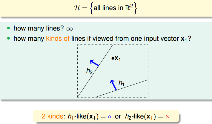
How Many Lines Are There?

|500 source: https://www.csie.ntu.edu.tw/~htlin/course/ml24fall/doc/05u_handout.pdf p.9

|500 source: https://www.csie.ntu.edu.tw/~htlin/course/ml24fall/doc/05u_handout.pdf p.12

|500 source: https://www.csie.ntu.edu.tw/~htlin/course/ml24fall/doc/05u_handout.pdf p.13

Effective Number of Lines

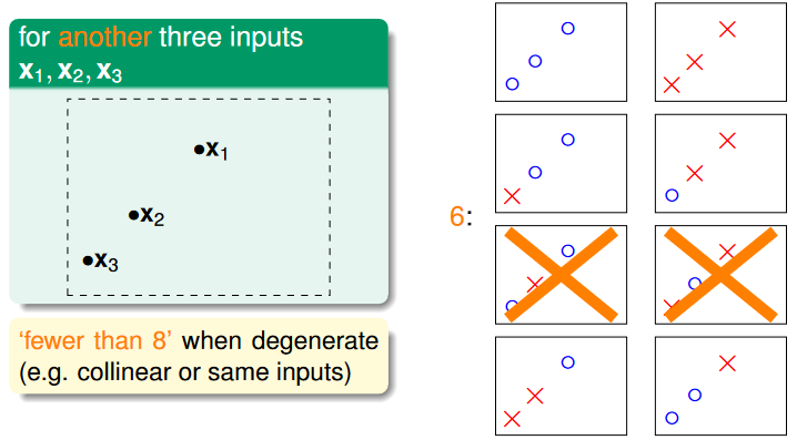
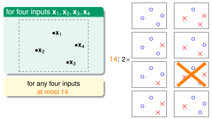
從上面可以發現，當有多個 inputs 的時候，我們必須考慮點重合在同一條線的情況，而我們將「 $N$ 個 inputs 最多能畫出來的線」叫做「effective number of lines」。

由於 effective number of lines 一定會小於等於 $2^N$ ，因此我們有機會將 infinite 的 $\mathcal{H}$ 歸納成 finite 數量的 group of $h$ ，這樣就能夠用 effective number 來代替原本的 $M$ (原本的公式):

$\mathbb{P}[|E_{\text{in}}(g) - E_{\text{out}}(g)| \gt \epsilon] \le 2\cdot\text{effective}(N)\cdot\exp\left(-2\epsilon^2N\right)$

Dichotomies

首先，我們將

$h({\bf x}_1,{\bf x}_2,\cdots,{\bf x}_N) = (h({\bf x}_1),h({\bf x}_2),\cdots,h({\bf x}_N)) \in \{\text{x}, \text{o}\}^N$

稱為 dichotomy，也就是限定 inputs 的 hypothesis。而 dichotomies

$\mathcal{H}({\bf x}_1,{\bf x}_2,\cdots,{\bf x}_N) = \{\text{all dichotomy}\ h({\bf x}_1,{\bf x}_2,\cdots,{\bf x}_N)\}$

則代表的就是所有對應 inputs 的 dichotomy 的集合。

所以我們可以用 dichotomies 的大小 $|\mathcal{H}({\bf x}_1,{\bf x}_2,\cdots,{\bf x}_N)|$ (有 upper bound $2^N$ ) 來代替原本 $\mathcal{H}$ 的大小 $M$ (可能是 infinte)。

Growth Function

由於 $|\mathcal{H}({\bf x}_1,{\bf x}_2,\cdots,{\bf x}_N)|$ 會跟 inputs 有關，所以我們計算時都會考慮最壞的情況，也就是取可能的最大值:

$m_{\mathcal{H}}(N) = \max_{{\bf x}_1,\cdots,{\bf x}_N\in\mathcal{X}}|\mathcal{H}({\bf x}_1,{\bf x}_2,\cdots,{\bf x}_N)|$

這個被叫做 growth function，也就是計算「當 input 成長時，dichotomies 的大小如何成長」。

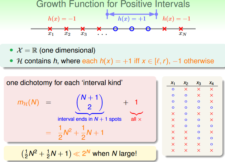
計算 growth function 的例子:

|500 source: https://www.csie.ntu.edu.tw/~htlin/course/ml24fall/doc/05u_handout.pdf p.17

|500 source: https://www.csie.ntu.edu.tw/~htlin/course/ml24fall/doc/05u_handout.pdf p.18

|500 source: https://www.csie.ntu.edu.tw/~htlin/course/ml24fall/doc/05u_handout.pdf p.20

|500 source: https://www.csie.ntu.edu.tw/~htlin/course/ml24fall/doc/05u_handout.pdf p.21

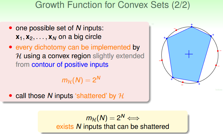
當 N 個 inputs 的任意組合 $\mathcal{H}$ 都有一個對應的 dichotomy 可以準確分類他們，也就是 $m_{\mathcal{H}}(N) = 2^N$ ，這時候我們就說這個 $\mathcal{H}$ 可以 shatter 這 N 個 inputs。

Break point

事實上，shatter 的情況是我們最不樂見的，這代表我們沒辦法「刪除」某些 input 組合來減少 dichotomy 的數量，因為每一種組合都可以被 $\mathcal{H}$ 分類。

現在來看看 2D perceptron 的例子:

$N = 1$ : 可以被 shatter
$N = 2$ : 部分情況可以被 shatter
$N = 3$ : 部分情況可以被 shatter
$N = 4$ : 沒有任何情況可以被 shatter (不管怎樣都只能找出 $14 \lt 2^4$ 種 dichotomy)

當 $k$ 個 inputs 的組合在任何情況下都不能被 shatter 時，也就是 $m_{\mathcal{H}}(k) \lt 2^k$ ，我們就說這個 $k$ 是 break point，像是 2D perceptron 的 break point 就是 $N = 4, 5, \cdots$ ，通常我們只會考慮最小的 break point。

統整前面提過的例子:


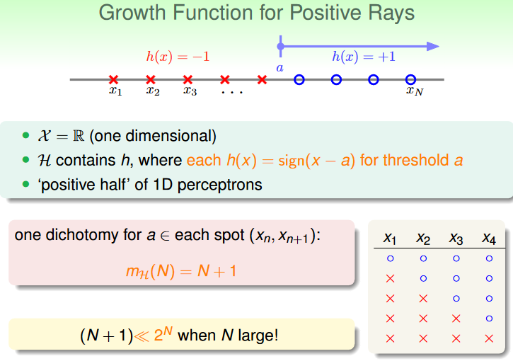
positive rays	break point at 2	$m_{\mathcal{H}}(N) = N+1 = O(N)$
positive intervals	break point at 3	$m_{\mathcal{H}}(N) = {1\over2}N^2 + {1\over2}N + 1 = O(N^2)$
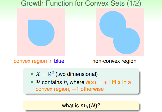
convex sets	no break point (不管 N 是多少都會被 shatter)	$m_{\mathcal{H}}(N) = 2^N$
2D perceptrons	break point at 4	$m_{\mathcal{H}}(N) \lt 2^N$ in some cases

可以發現當有 break point $k$ 的時候， $m_{\mathcal{H}}(N) = O(N^{k-1})$ ，這部分的證明在 lecture 6 (教授說是 optional，所以我就沒有做筆記了)。